Notes about Crash course in Machine Learning

Following this [Machine Learning - Crash Course](https://developers.google.com/machine-learning/crash-course/
License)

Licensed under CC 3.0

Framing: Key ML Terminology

supervised machine learning - learns based on input data how to make predictions on unseen data

Terminology

• Label - what we are predicting (y variable in simple linear regression)
• Feature - input variable (words, faces, time, data) (x variable)
• Examples
  • labeled (used to train the model) {features, label}: (x, y)
  • unlabeled (used to predict) {features, ?}: (x, ?)
• Model - defines the relationship between features and labels
  • training means teaching or learning the model
  • inference means applying the model on unlabeled examples
• Regression vs classification
  • regression model predict continuous values (house prices, probability)
  • classification model predicts discrete values (spam_not-spam, image is cat_dog)

Descending into ML

Linear regression

A linear relationship is defined by the linear regression equation:

$$
y = mx + b
$$

Where y is the predicted value, m is the slope of the line, x is the value of input and b is also called the y-intercept, the initial “offset” of your function.

In ML, it is slightly different:

$$
\hat{y} = w_1 x_1 + b
$$

Again, y' is the predicted output value, w1 is the weight associated to each feature (x-value), x1 is the first feature and b is also called the bias, also referred to as w0 (weight of the first feature).

Training and loss

Training means determining good (predicted) values for a certain feature (labelled example). To find a good model you’ll need to reduce the loss for each prediction by feeding it many good examples. This is called “empirical risk minimisation”. The closer the loss is for each prediction, the better the trained model is.

A popular loss function to determine this is “Mean Squared Error“, where you compute the “square of the difference between the label and the prediction” and apply it to every datapoint of the labelled examples.

$$
1 / N * \sum_{(x,y) \in D}{ } (y - prediction(x))^2
$$

You can also read the y variable as “observation”, the value of the labelled example.

It is to be said, that MSE is not the only loss function that can be used, there are others and better.

Reducing loss

An iterative approach

To reduce and the determine the loss while iterating our data set, often a technique called “Gradient Descent” is used. It takes an iterative approach to train the model.

It comes from Calculus and applied to machine learning an adapted version of it is used: “mini-batch gradient descent” (Gradient Descent). In other words, instead of taking the whole data set to compute the loss function, we take a mini batch of it for training our model, and another one to to see if the loss was reduced or not on the prediction. The starting values for each weight / loss are not so important (usually set to 0), since the Machine learning algorithm will at each iteration update this parameters and (ideally) get better results with more features to train on.

The algorithm will iterate over the data set and find the lowest possible loss. At this point, the model has converged

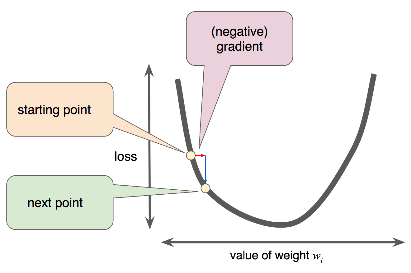
Gradient Descent

Note that a gradient is a vector, so it has both of the following characteristics:

• a direction
• a magnitude

Gradient descent relies on negative gradients to determine the next lowest loss for the model. It works for convex machine learning problems.

Learning rate

As mentioned above, Gradients are vectors, thus the have to important properties: direction and magnitude. In gradient descent algorithms you’ll multiply the gradient by a scalar, also known as the learning rate (“step size”).
The learning rate is one of the Hyperparameters used used to tweak machine learning algorithms.
There is also a principle called Goldilocks which is used to determine a neither too small nor too big learning rate-